PathTracer

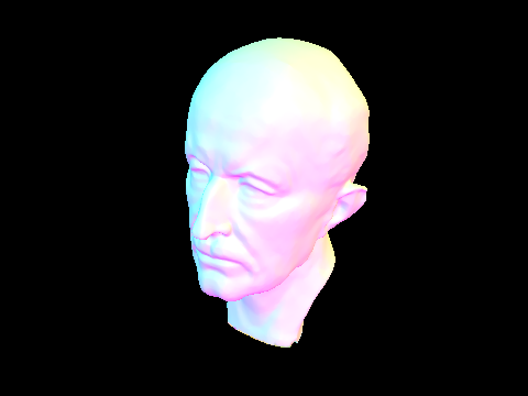
In this project we have implemented the important functions which are necessary for a ray tracing method. This includes generating a number of rays inside a [0,1]*[0,1] box for each pixel and projecting them to the camera view in our scene which is in the world coordinates. Then, this rays should be followed in the scene to check for intersection. In part 1 of the prjection we check the intersection between each ray genrated and all the mesh triangle in the scene for intersection which is time consuming and return the closest intersection as a spectrum which include the color of the pixel. This should be done for all sample rays for a pixel and the averaged value over all sample rays is the final spectrum passed to a pixel to be shown. In part 2 we try to improve method using bounding box trees; it is done by dividing all the primitives(triangles, circles, ...) to sub bodnding boxes of a tree structure and testing each sample to see if there is an intersetion between a bounding box and the ray. This helps to efficiently find the primitives that a ray is actually intersecting with and we will be able to efficiently do the ray tracing for more complicated shapes. To be able to show the results for the first two part we used normal vector of each primitive at the point to get a spectrum for the poing and use this spectrum as the colore of the pixel to show.

In part 3 we focus on direct ilumination for diffuse BSDF materials. When a rays hits a primitive in the scene we sample some outgoing rays to intersect with the enviroment using Monte Carlo integration and collect the incoming light to the hit point and using the BSDF properties of the hit point we return a spectrum for the color of the hit point and it passes to the pixel. Part 4 is there to take care of indirect lighting. When a ray hit point and we use incoming radiances from other points to get color at a point, this incoming rays can by themselve come from a another points and we can do direct lighinng for these sets of points and then use them for the first hit point. This can goes on and on recursively. Thus, we use a termination method to get the last set of rays and turn them back until we get to the firs het point in the scene and use the combined color to be shown on the scene. Part 5 is devoted to find the averaged spectrum of the incoming sample rays to a pixel and use statistics to conclude if the color of the specified pixel is convereged to right value or not and if this is the case it will prevent the system from sending extra rays for a specific pixel to do the ray tracing and this way we can get a more efficient code.

Part 1: Ray Generation and Intersection

For this part we generate a number of points randomly in a rectangular domain of [0,1]^2 to hit the specified pixel, this is using a defined gridsampler function. Then, these points are converted to camera view to generate rays using the vertical and horizontal field of view, which are angle of vies in camera, from the coordinate on the pixel to the camera coodinate. Then we convert this point to world corrdinate by construcing a Vector3D for point on the camera. Afterward, we generate a ray using this direction that we determined in world coordinates and the positon that we have the field of view or eye. We should also fix the limits of the this ray which depend on the camera position in the world.

Now that the ray is generated we should find how this ray is intersecting with a primitive. The most common one is triangle primitives that we discuss it here to how find the solution.

To find the intersection between a ray and a triangle we use a barycenteric representation for points inside the triangle using three vertices.

P = b1*p1+b2*p2+b3*p3

Where p1, p2 and p3 are triangle points and b1,b2 and b3(b1+b2+b3=1) are barycenteric coordinates. And another representation for the ray

P = o + t*d

where o is the orgin of the ray and d is the direction and t is constant limit by camera view. These two points intersct at one specific point os they sould be eqaul. Solving for b1, b2 and t(b3 is a function b1 and b2) we can find these values.

o+t*d = b1*p1+b2*p2+(1-b1-b2)*p3

or

-t*d+b1*(p1-p3)+b2*(p2-p3) = o-p3

Since these are 3D vectors then there are 3 equation for three unknown t, b1 and b2. lets call S = o-p3, e1 = p1-p3, e2 = p2-p3.

-t*d+b1*e1+b2*e2 = s, [-d,e1,e2]*[t,b1,b2]^T= s

We know that the solution for this system of equation based on cramer ruls is:

t = det[s,e1,e2]/det[-d,e1,e2], b1 = det[-d,s,e2]/det[-d,e1,e2], b2 = det[-d,e1,s]/det[-d,e1,e2]

or

t = cross(s,e1).e2/cross(d,e2).e1, b1 = cross(d,e2).s/cross(d,e2).e1, b2 = cross(s,e1).d/cross(d,e2).e1

If we replace:

cross(s,e1) = s2, cross(d,e2) = s1

then we have,

 t = s2.e2/s1.e1, b1 = s1.s/s1.e1, b2 = s2.d/s1.e1

and this is how we set obtain the unknowns in the code. Then we determine if the intersection is valid using the bouding of the variable t and if b1, b2 and b3 are positive. If that is the case; then, we set the properties of an Intersection object such as which primitive is included in the interstion, what is the normal at that point, and in what t the interstion is happend, and we set maximum value for t to be equal to the new value that we detemined.

For a sphere we also follow the same roles suggested in the class on how to determine the number of intersection and choose which on is the closest based on the distance and finally set the interstion object properties accoringly.

Below we can see some simple examples of the normal shading.

Part 2: Bounding Volume Hierarchy

BVH construction algorithm: to organize all primitives inside a tree structure of bounding box we use a recursive method to start from a large bounding box that incloses all the primitives in the scene, this boundig box has two left and right childs and a vector of primitives. Then, we want to split the box in a way that around half of the primitives are stored in the right child bounding box and half of them in the left child bounding box. We do this for childs also to finally get the number of primitives in the bounding box to be less than the determined size. In order to be able to split the large bounding boxes we define another bounding box called centriod_box to store the center of all the bounding box of the primitives in it. In this way when we want to split the prvimitive we use the center of this centriod_box and it guarantees that we have primitives in left and right childs and there is no problem regarding having an infinte loop due to and empty child for the bounding box.

Then we implement the algorithm for ray intersecting a bounding box to be used in the accelerated BVH alogrithm. This is a simple a way to check if a ray intersect with a box or not; which helps to avoid extra intersections for all primitives inside the box.

BVH intersection algorithm: In this algorithm we first check to see if the incoming ray intersect with the given bounding box. If it does not we return false since there is no intersection otherwise we check if there is any primitive inside the bounding box. If there is any we check for intersection with primitives and we return true if there is one other wise we should repeat the intersection check for both the left and right child inside the bounding box and we call the same intersection function inside these functions so it is recursive method.

Below we have shown the results for two cases of comlicated shapes for rendering.

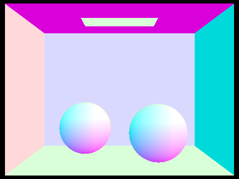
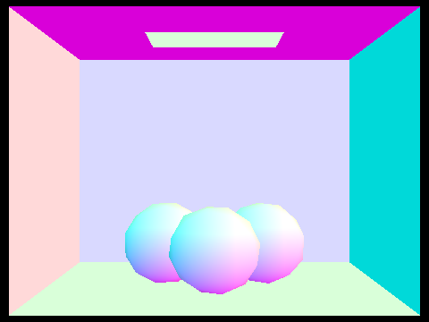
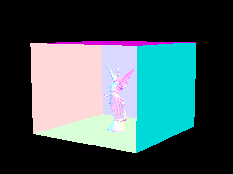
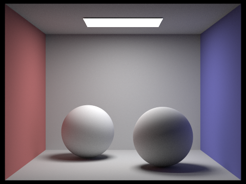
Part 3: Direct Illumination

First of all we set the reflectance and probability densidy function for a diffuse BSDF material inside the related function.

Here we have a function to take care of direct lighting. In this function we pass the hit point and the ray that comes from the camera. Then we define these variables in world and object component. Now to pass a spectrum to pixel that ray is coming from we should send out a number of ray from the hit point to the scene light. For this purpose we loop over all the scene lights and find out if it is a delta light or not. If it is not a delta light we need one sample light from it because it is just a oint light otherwise we need to get a number of sample from it since the lighe is covering an area in the scene. After having the sample light we have the inforamtion regarding the distance between hit point and the light and the incoming light direction. Thus we can check for the incoming radiang to get the correct spetrum after taking care of cosine terms and probability density function. After collecting all of these sample spectrum we get the average spcetrum and combined it with diffuse BSDF properties of the hit point we return the final value of the direct lighing for the pixel.

Below there are a number of images with direc illuminatioin:

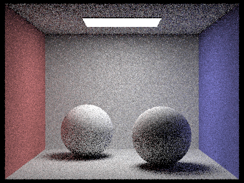
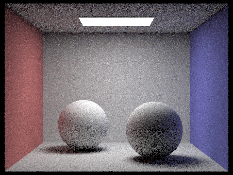
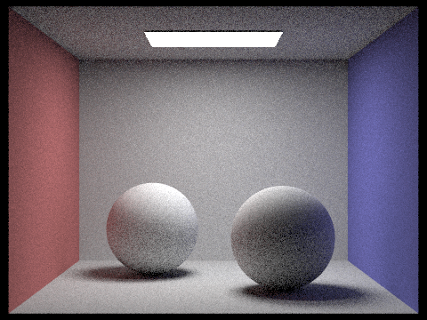
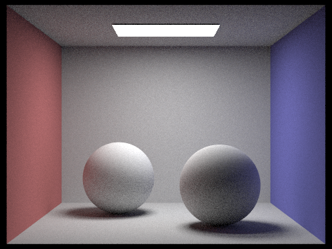
Below there are a number of images with direct illuminatioin with 1, 4, 16, and 64 light rays:

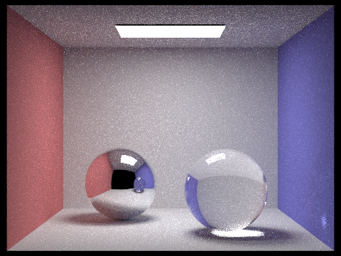
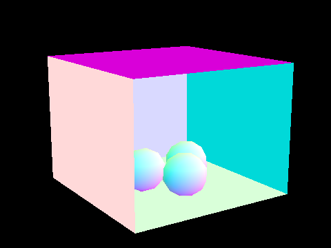
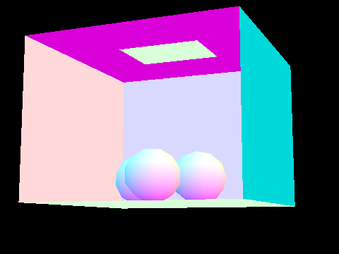
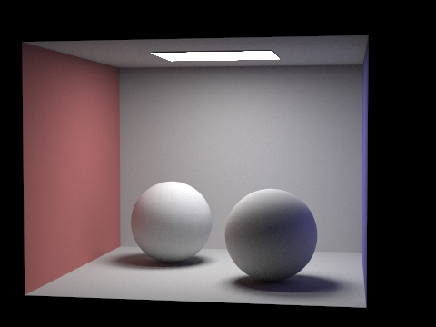
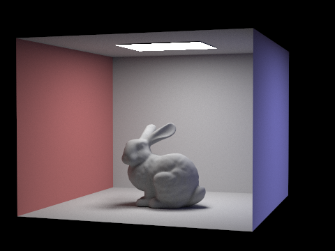
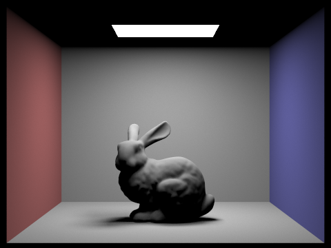
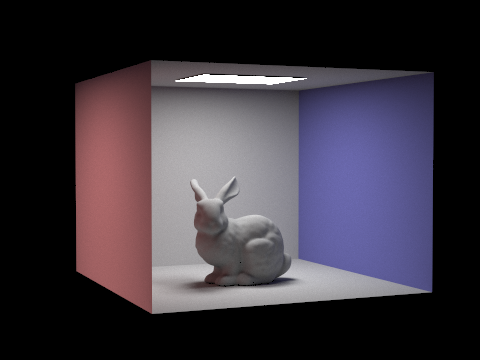
Part 4: Indirect Illumination

Here we continue what we have done for direct lighting in a recursive way. When a ray hits a primitive we first get direct lighting; then, in a function for indirect lighting we measure the illumination of the hit surfce and determine if the illumination is large enough to sample from the incoming radiance and add another spectrum to the system. If the illlumination passes a threshold; then, we get random incoming radiace and track it using calling trace_ray() function and compute the incoming radiance from this ray. The same ray may again go through this process to collect spectrum from other incoming radiances. These process goes on and on untill the ilumination of the hit point is negiligble. Afterward, the code sum up all the spectrums together and return the indirect lighting for the pixel.

Below we can see two examples of direct and indirect illumination together,

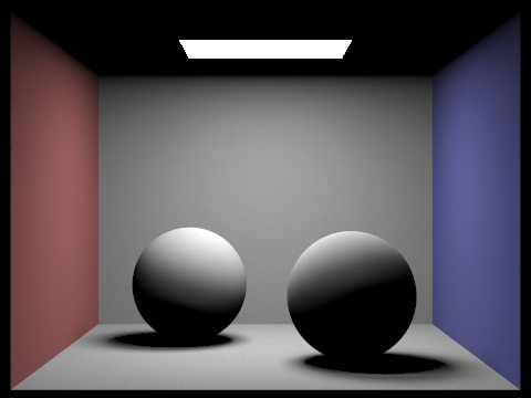
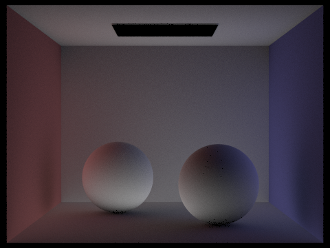
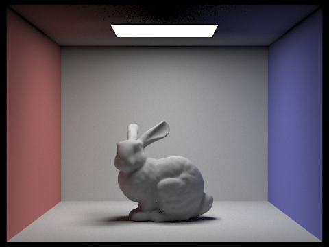
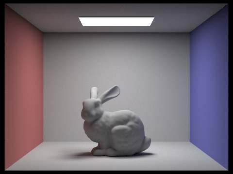
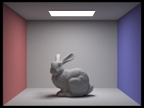
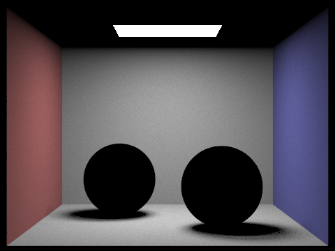
Below we can see a scene with only direct illumination and another one with only indirect illumination:

Below we can see a scene with max_depth_ray 0,1,2,3,100:

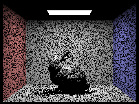
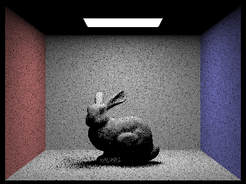
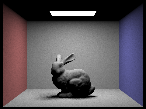
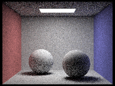
Below we can see a scene with sample-per pixel for 1,2,4,8,16,64,1024

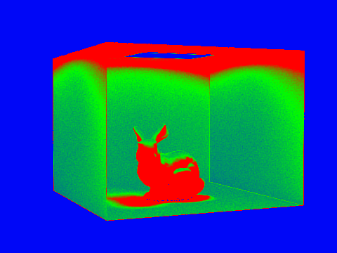
Part 5: Adaptive Sampling

To implement this part we define a set of variables for later use. s1 and s2 are used to store the summation of illumination of a each sample ray for a pixel and illumination square. Then, the mean(mu) and standard deviation(sigma) of the illumination of all the sample points is computed every 32 time. Afterward, it is needed to compute the variable I = 1.96*sigma/sqrt(n) and compare it with maxTolerance*mu. If the value is less than the tolerance we can terminate sampling for the pixel since the value of illumination is close to a specific value and its deviation is small enough to assume that the function converged.

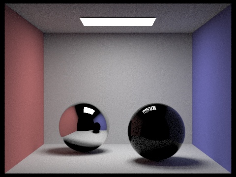
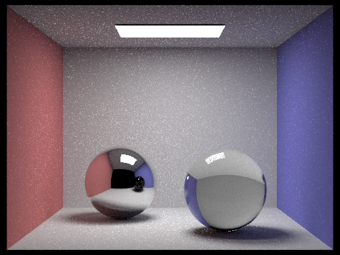
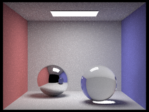
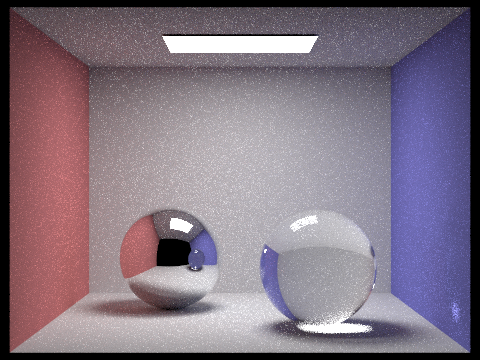
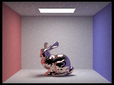
Part 6: Mirror and Glass Materials

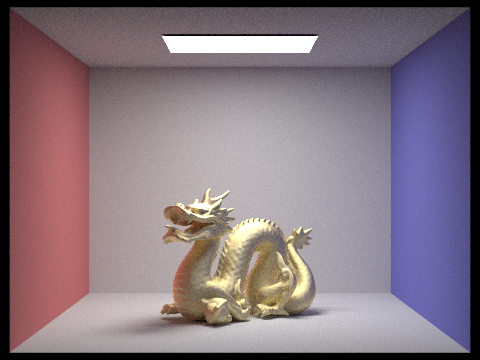
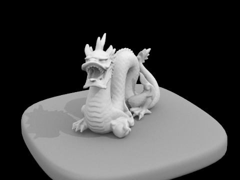
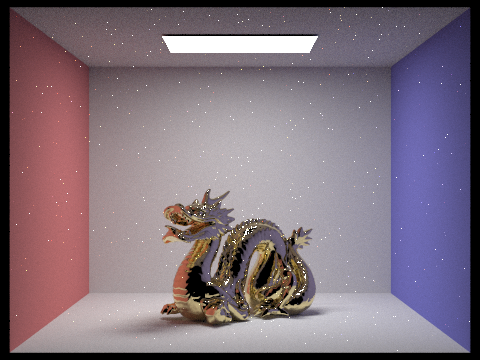
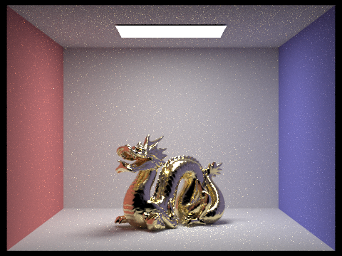
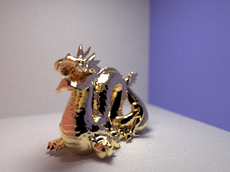
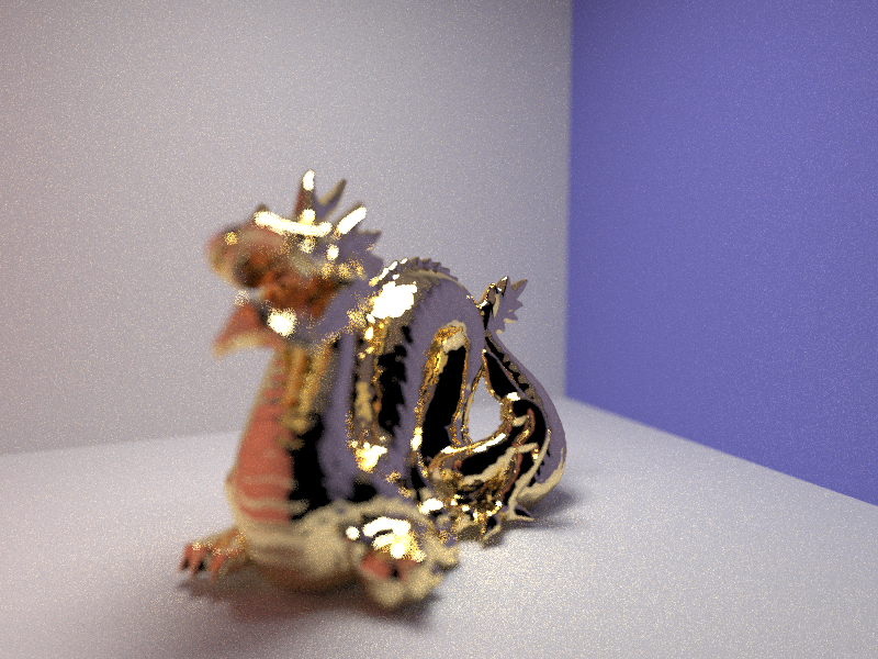
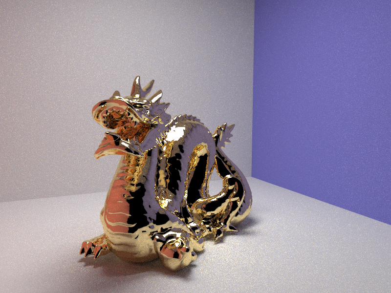
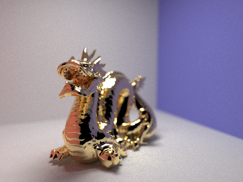
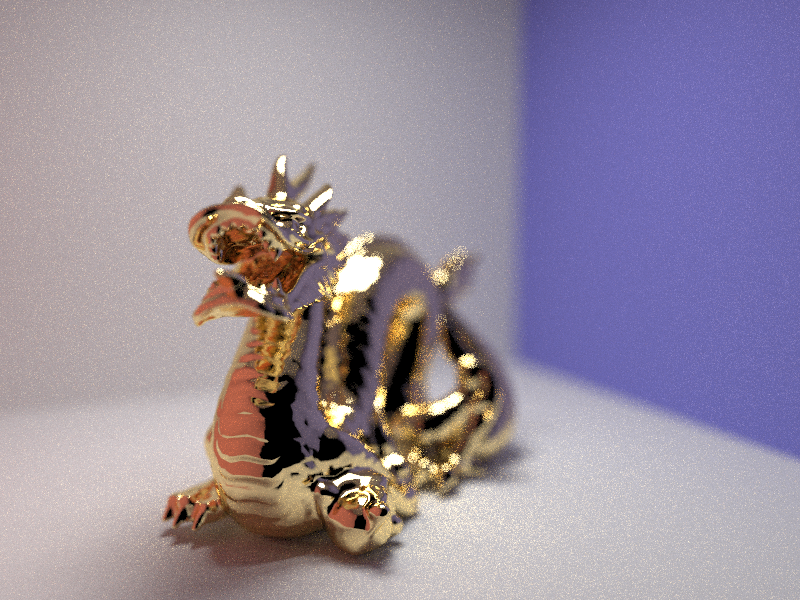
Part 7: Microfacet Material

For the dragon as it is shown below for smaller alphas we have a smoother surface. Alpha has been used to find the distribution of the normals at the hitting points. As alpha get larger this distibution gets expanded to wider range of normal which are different than from real normal to the surface. And as alpha gets smaller the corresponding sampled normals ar closer the real normal to the surface and the matreial looks more glossy.

To compare cosine hemisphere sampling and importance sampling. The reslut for importance sampling is birther and less noisy.

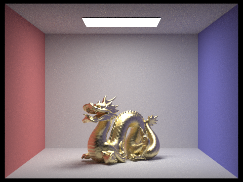
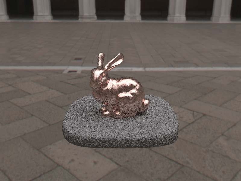
Using lead as a material for rendering we get this: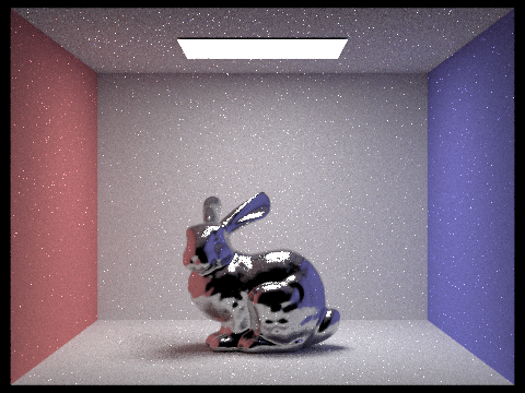

Part 8: Environment Light

The corresponding probability distribuition for doge.exr file is shown below.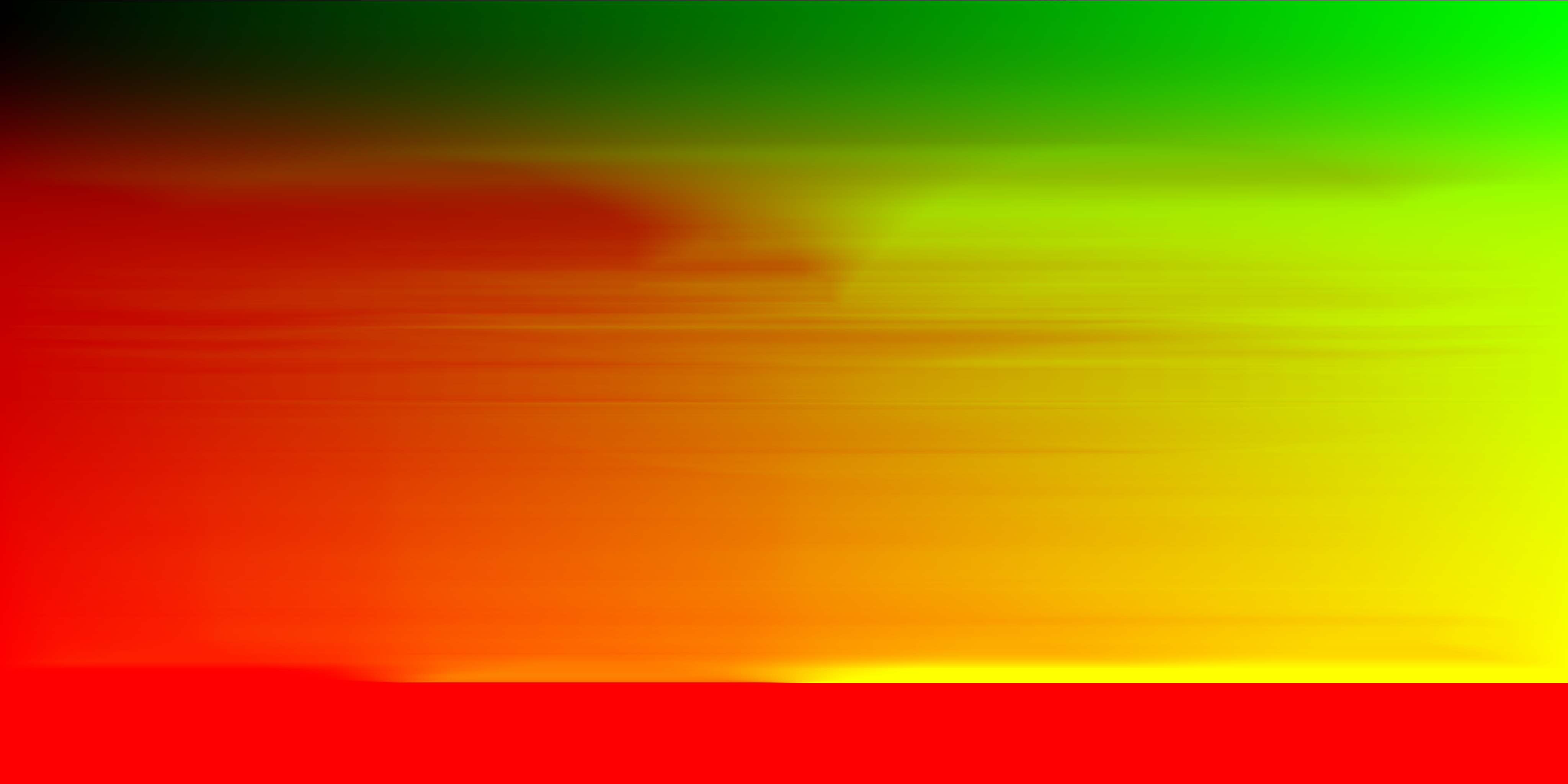

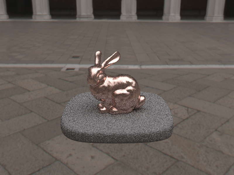
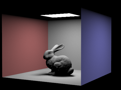
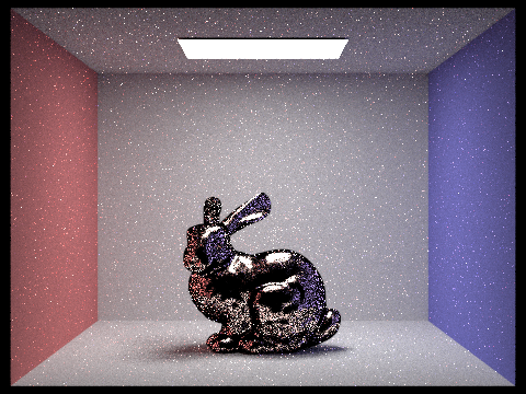
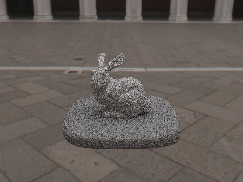
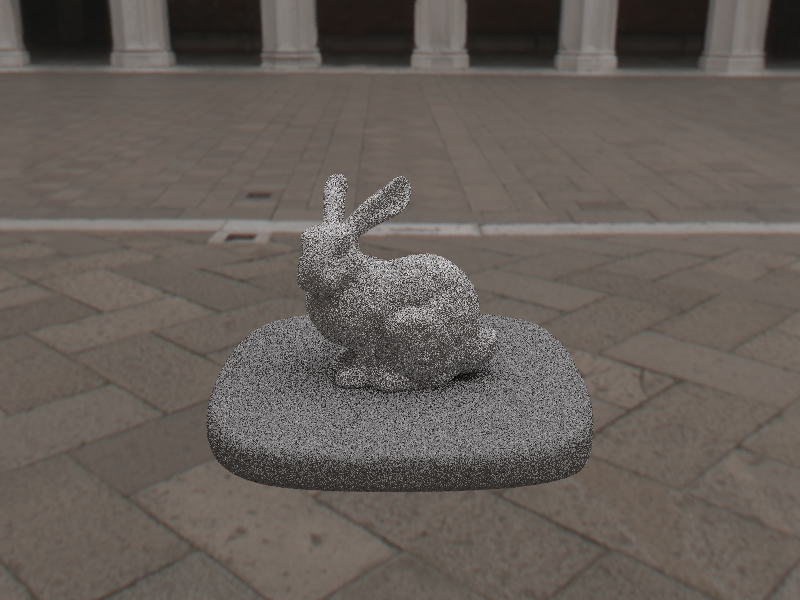
Below we have shown the reulsts for bunny_unlit.dae using uniform sampling and importance sampling, as we can see the case with importance sampling is less noisy.

Below we have shown the reulsts for bunny_microfacet_cu_unlit.dae using uniform sampling and importance sampling, as we can see the case with importance sampling is less noisy.

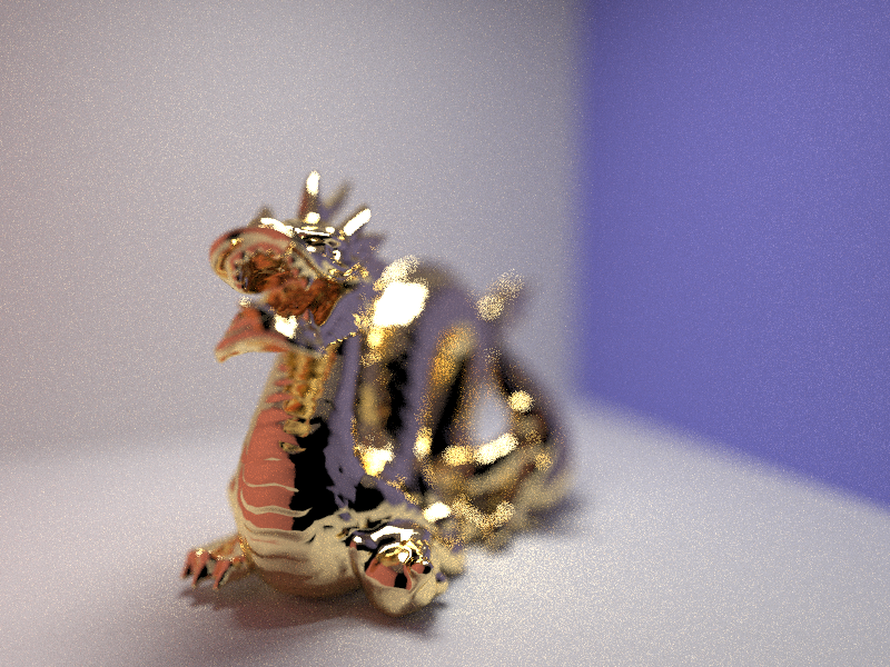
Part 9: Depth of Field

Here we show a stack of 4 picture for CBdragon for different depth of field and same lens radius,

Here we show a stack of 4 picture for CBdragon for with visibly different aperture sizes and same depth of field,